The Standardized Precipitation Index (SPI) is a tool used to quantify precipitation deficits for different time scales. It’s particularly useful in drought assessments where understanding the intensity and duration of dry spells is critical. SPI is calculated by fitting precipitation data to a probability distribution, which is then normalized so that the index has a mean of zero and a standard deviation of one. The SPI can be calculated over various scales, typically ranging from 1 month to 48 months, reflecting the impact on different water resources. To understand how SPI is calculated, you can read our blog.
Data Requirements for SPI Calculation
To calculate the SPI effectively, you need:
- Precipitation Data: Monthly precipitation data for the location of interest. The data should be in a vector format (single column with each entry representing monthly total precipitation).
- Length of Data: A minimum of 30 years of data is recommended to ensure statistical reliability. More data would provide a more robust fit to the statistical model.
- Scale: The time scale in months over which the SPI is calculated. Common scales are 1, 3, 6, 12, and 24 months, but it can be extended up to 48 months.
The MATLAB Function for SPI Calculation
Below is a MATLAB function designed to compute the SPI for monthly precipitation data without the need for specifying the number of seasons, as we will assume monthly data handling. This function calculates SPI by fitting data to a gamma distribution and then transforming it to a Z-score.
Example Usage
we will demonstrate how to compute and visualize various Standardized Precipitation Index (SPI) time series using MATLAB. This example focuses on SPI calculations at multiple scales for precipitation data from Texas Climate Division 9. The data is from 1982 to 2016.
The data used in this analysis consists of monthly precipitation records. The first two columns of the dataset represent the year and month, respectively, while the third column contains the precipitation amounts. You can view and download the dataset from my github repo.
We calculate the SPI for five different scales: 1, 3, 6, 12, and 24 months. These scales allow us to analyze drought conditions at various timeframes, from short-term impacts to long-term trends.
spi_timeseries now contains five columns, each representing a different SPI time series corresponding to the scales defined in the scale array.
We will now plot each SPI time series in a separate subplot for easy comparison. This visualization helps in understanding how drought conditions evolve over different time scales.
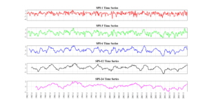
Figure: The SPI-time series generated for the Climate Division-9, Texas.
Key Points in the Script
- Data Loading and Processing: We load the precipitation data and extract the necessary columns for further analysis.
- SPI Calculation: We loop over the specified scales and compute the SPI for each, storing the results in a matrix.
- Visualization: We use subplots to display each SPI time series, allowing for comparisons across different scales.